Covariance Processing example

Introduction

This example is taken from Listing S10 in the 2013 JBNMR nmrglue paper. In this example covaraince processing is performed on a 2D NMRPipe file.

Instructions

The test.ft file is provided in the archive. To create this from time domain data use the NMRPipe script x.com

Execute python cov_process.py to perform the covariance processing on the test.ft file. The file test.ft2 is created.

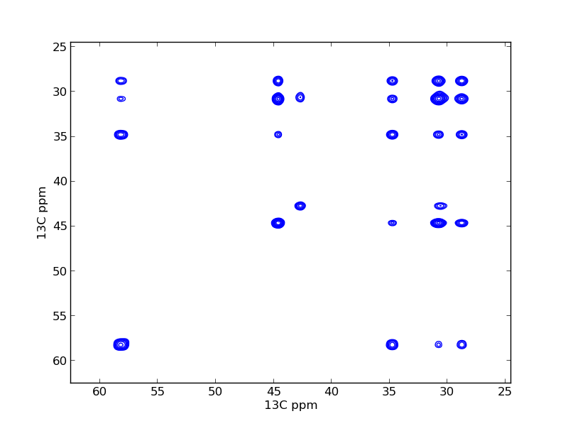
Execute python cov_plot.py to perform the covariance processing and plot the results. The output, covariance_figure.png is presented as Figure 5 in the article.

The data used in this example is available for download.

Listing S10

[cov_process.py]

import nmrglue as ng
import numpy as np

# open the data
dic, data = ng.pipe.read("test.ft")

# compute the covariance
C = np.cov(data.T).astype('float32')

# update the spectral parameter of the indirect dimension
dic['FDF1FTFLAG'] = dic['FDF2FTFLAG']
dic['FDF1ORIG'] = dic['FDF2ORIG']
dic['FDF1SW'] = dic['FDF2SW']
dic["FDSPECNUM"] = C.shape[1]

# write out the covariance spectrum
ng.pipe.write("test.ft2", dic, C, overwrite=True)

[cov_plot.py]

import nmrglue as ng
import matplotlib.pyplot as plt
import numpy as np

# open the data
dic, data = ng.pipe.read("test.ft")
uc = ng.pipe.make_uc(dic, data, 1)
x0, x1 = uc.ppm_limits()

# compute the covariance
C = np.cov(data.T)

# plot the spectrum
fig = plt.figure()
ax = fig.add_subplot(111)
cl = [1e8 * 1.30 ** x for x in range(20)]
ax.contour(C, cl, colors='blue', extent=(x0, x1, x0, x1), origin=None)
ax.set_xlabel("13C ppm")
ax.set_xlim(62.5, 24.5)
ax.set_ylabel("13C ppm")
ax.set_ylim(62.5, 24.5)
plt.savefig('covariance_figure.png')