3D strip plot example
Introduction
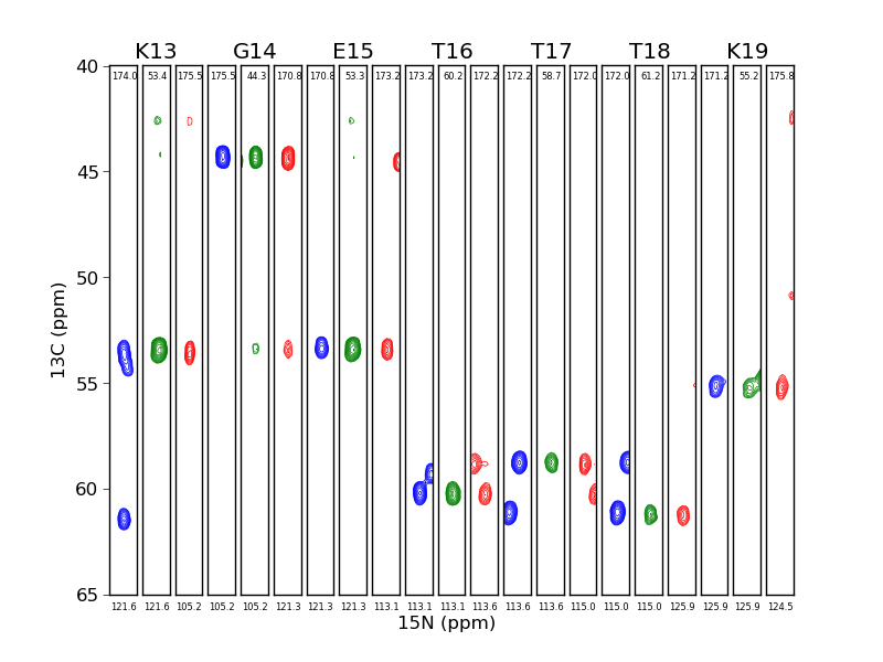
This example is taken from Listing S11 from the 2013 JBNMR nmrglue paper. In this example a three 3D solid state NMR spectra are visualized as strip plots.
Instructions
Process each of the three 3D spectra by decending into the appopiate directory and executing the fid.com followed by the xy.com NMRPipe scripts.
Execute python make_strip_plots.py to create the strip plots. The resulting file strip_plots.png is presented as Figure 6 in the paper.
The data used in this example is available for download part1, part2.
Listing S11
#! /usr/bin/env python

import nmrglue as ng
import numpy as np
import matplotlib.pyplot as plt

# NMRPipe files of spectra to create strip plots from
spectrum_1 = 'GB3-CN-3DCONCA-041007.fid/ft/test%03d.ft3'
spectrum_2 = 'GB3-CN-3DNCACX-040507.fid/ft/test%03d.ft3'
spectrum_3 = 'GB3-CN-3DNCOCX-040807.fid/ft/test%03d.ft3'

# contour parameters
contour_start_s1 = 1.0e5
contour_step_s1 = 1.15

contour_start_s2 = 2.3e5
contour_step_s2 = 1.15

contour_start_s3 = 3.0e5
contour_step_s3 = 1.20

colors_s1 = 'blue'
colors_s2 = 'green'
colors_s3 = 'red'

cl_s1 = contour_start_s1 * contour_step_s1 ** np.arange(20)
cl_s2 = contour_start_s2 * contour_step_s2 ** np.arange(20)
cl_s3 = contour_start_s3 * contour_step_s3 ** np.arange(20)

# open the three data sets
dic_1, data_1 = ng.pipe.read_lowmem(spectrum_1)
dic_2, data_2 = ng.pipe.read_lowmem(spectrum_2)
dic_3, data_3 = ng.pipe.read_lowmem(spectrum_3)

# make unit conversion objects for each axis of each spectrum
uc_s1_a0 = ng.pipe.make_uc(dic_1, data_1, 0)  # N
uc_s1_a1 = ng.pipe.make_uc(dic_1, data_1, 1)  # CO
uc_s1_a2 = ng.pipe.make_uc(dic_1, data_1, 2)  # CA

uc_s2_a0 = ng.pipe.make_uc(dic_2, data_2, 0)  # CA
uc_s2_a1 = ng.pipe.make_uc(dic_2, data_2, 1)  # N
uc_s2_a2 = ng.pipe.make_uc(dic_2, data_2, 2)  # CX

uc_s3_a0 = ng.pipe.make_uc(dic_3, data_3, 0)  # CO
uc_s3_a1 = ng.pipe.make_uc(dic_3, data_3, 1)  # N
uc_s3_a2 = ng.pipe.make_uc(dic_3, data_3, 2)  # CX

# read in assignments
table_filename = 'ass.tab'
table = ng.pipe.read_table(table_filename)[2]
assignments = table['ASS'][1:]

# set strip locations and limits
x_center_s1 = table['N_PPM'][1:] # center of strip x axis in ppm, spectrum 1
x_center_s2 = table['N_PPM'][1:] # center of strip x axis in ppm, spectrum 2
x_center_s3 = table['N_PPM'][2:] # center in strip x axis in ppm, spectrum 3
x_width = 1.8               # width in ppm (+/-) of x axis for all strips

y_min = 40.0   # y axis minimum in ppm
y_max = 65.0   # y axis minimum in ppm

z_plane_s1 = table['CO_PPM'][:]   # strip plane in ppm, spectrum 1
z_plane_s2 = table['CA_PPM'][1:]  # strip plane in ppm, spectrum 2
z_plane_s3 = table['CO_PPM'][1:]  # strip plane in ppm, spectrum 3


fig = plt.figure()
for i in xrange(7):

    ### spectral 1, CONCA
    # find limits in units of points
    idx_s1_a1 = uc_s1_a1(z_plane_s1[i], "ppm")
    min_s1_a0 = uc_s1_a0(x_center_s1[i] + x_width, "ppm")
    max_s1_a0 = uc_s1_a0(x_center_s1[i] - x_width, "ppm")
    min_s1_a2 = uc_s1_a2(y_min, "ppm")
    max_s1_a2 = uc_s1_a2(y_max, "ppm")

    if min_s1_a2 > max_s1_a2:
        min_s1_a2, max_s1_a2 = max_s1_a2, min_s1_a2

    # extract strip
    strip_s1 = data_1[min_s1_a0:max_s1_a0+1, idx_s1_a1, min_s1_a2:max_s1_a2+1]

    # determine ppm limits of contour plot
    strip_ppm_x = uc_s1_a0.ppm_scale()[min_s1_a0:max_s1_a0+1]
    strip_ppm_y = uc_s1_a2.ppm_scale()[min_s1_a2:max_s1_a2+1]
    strip_x, strip_y = np.meshgrid(strip_ppm_x, strip_ppm_y)

    # add contour plot of strip to figure
    ax1 = fig.add_subplot(1, 21, 3 * i + 1)
    ax1.contour(strip_x, strip_y, strip_s1.transpose(), cl_s1,
                    colors=colors_s1, linewidths=0.5)
    ax1.invert_yaxis()  # flip axes since ppm indexed
    ax1.invert_xaxis()

    # turn off tick and labels, add labels
    ax1.tick_params(axis='both', labelbottom=False, bottom=False, top=False,
                    labelleft=False, left=False, right=False)
    ax1.set_xlabel('%.1f'%(x_center_s1[i]), size=6)
    ax1.text(0.1, 0.975, '%.1f'%(z_plane_s1[i]), size=6,
                                        transform=ax1.transAxes)

    # label and put ticks on first strip plot
    if i == 0:
        ax1.set_ylabel("13C (ppm)")
        ax1.tick_params(axis='y', labelleft=True, left=True, direction='out')

    ### spectra 2, NCACX
    # find limits in units of points
    idx_s2_a0 = uc_s2_a0(z_plane_s2[i], "ppm")
    min_s2_a1 = uc_s2_a1(x_center_s2[i] + x_width, "ppm")
    max_s2_a1 = uc_s2_a1(x_center_s2[i] - x_width, "ppm")
    min_s2_a2 = uc_s2_a2(y_min, "ppm")
    max_s2_a2 = uc_s2_a2(y_max, "ppm")

    if min_s2_a2 > max_s2_a2:
        min_s2_a2, max_s2_a2 = max_s2_a2, min_s2_a2

    # extract strip
    strip_s2 = data_2[idx_s2_a0, min_s2_a1:max_s2_a1+1, min_s2_a2:max_s2_a2+1]

    # add contour plot of strip to figure
    ax2 = fig.add_subplot(1, 21, 3 * i + 2)
    ax2.contour(strip_s2.transpose(), cl_s2, colors=colors_s2, linewidths=0.5)

    # turn off ticks and labels, add labels and assignment
    ax2.tick_params(axis='both', labelbottom=False, bottom=False, top=False,
                    labelleft=False, left=False, right=False)
    ax2.set_xlabel('%.1f'%(x_center_s2[i]), size=6)
    ax2.text(0.2, 0.975, '%.1f'%(z_plane_s2[i]), size=6,
                                        transform=ax2.transAxes)
    ax2.set_title(assignments[i])

    ### spectral 3, NCOCX
    # find limits in units of points
    idx_s3_a0 = uc_s3_a0(z_plane_s3[i], "ppm")
    min_s3_a1 = uc_s3_a1(x_center_s3[i] + x_width, "ppm")
    max_s3_a1 = uc_s3_a1(x_center_s3[i] - x_width, "ppm")
    min_s3_a2 = uc_s3_a2(y_min, "ppm")
    max_s3_a2 = uc_s3_a2(y_max, "ppm")

    if min_s3_a2 > max_s3_a2:
        min_s3_a2, max_s3_a2 = max_s3_a2, min_s3_a2

    # extract strip
    strip_s3 = data_3[idx_s3_a0, min_s3_a1:max_s3_a1+1, min_s3_a2:max_s3_a2+1]

    # add contour plot of strip to figure
    ax3 = fig.add_subplot(1, 21, 3 * i + 3)
    ax3.contour(strip_s3.transpose(), cl_s3, colors=colors_s3, linewidths=0.5)

    # turn off ticks and labels, add labels
    ax3.tick_params(axis='both', labelbottom=False, bottom=False, top=False,
                    labelleft=False, left=False, right=False)
    ax3.set_xlabel('%.1f'%(x_center_s3[i]), size=6)
    ax3.text(0.1, 0.975, '%.1f'%(z_plane_s3[i]), size=6,
                                        transform=ax3.transAxes)

# add X axis label, save figure
fig.text(0.45, 0.05, "15N (ppm)")
fig.savefig('strip_plots.png')