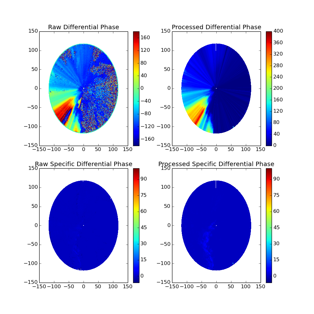
Linear programming phase processing

An example of using linear processing to process the differential phase fields of a ARM C-SAPR radar.

• 
• 

Script output:

Unfolding
Unfolding
Exec time:  13.6145980358
Doing  0

Python source code: plot_lp_phase_proc.py

print __doc__

# Author: Jonathan J. Helmus (jhelmus@anl.gov)
# License: BSD 3 clause

import numpy as np
import matplotlib.pyplot as plt
import pyart


# perform LP phase processing (this takes a while)
radar = pyart.io.read_mdv('095636.mdv')

# the next line force only the first sweep to be processed, this
# significantly speeds up the calculation but should be commented out
# in production so that the entire volume is processed
radar.sweep_start_ray_index['data'] = np.array([0])

phidp, kdp = pyart.correct.phase_proc_lp(radar, 0.0, debug=True)
radar.add_field('proc_dp_phase_shift', phidp)
radar.add_field('recalculated_diff_phase', kdp)

# the following line can be used to save/load in preprocessed data
#pyart.io.write_cfradial('preprocessed.nc', radar)
#radar = pyart.io.read_cfradial('preprocessed.nc')

# create a plot of the various differential phase fields
display = pyart.graph.RadarDisplay(radar)
fig = plt.figure(figsize=(10, 10))
ax1 = fig.add_subplot(221)
display.plot_ppi('differential_phase', 0, ax=ax1,
                 title='Raw Differential Phase', colorbar_label='',
                 axislabels_flag=False)

ax2 = fig.add_subplot(222)
display.plot_ppi('proc_dp_phase_shift', 0, ax=ax2,
                 title='Processed Differential Phase', colorbar_label='',
                 axislabels_flag=False)

ax3 = fig.add_subplot(223)
display.plot_ppi('specific_differential_phase', 0, ax=ax3,
                 title='Raw Specific Differential Phase', colorbar_label='',
                 axislabels_flag=False)

ax4 = fig.add_subplot(224)
display.plot_ppi('recalculated_diff_phase', 0, ax=ax4,
                 title='Processed Specific Differential Phase',
                 colorbar_label='',
                 axislabels_flag=False)
plt.show()

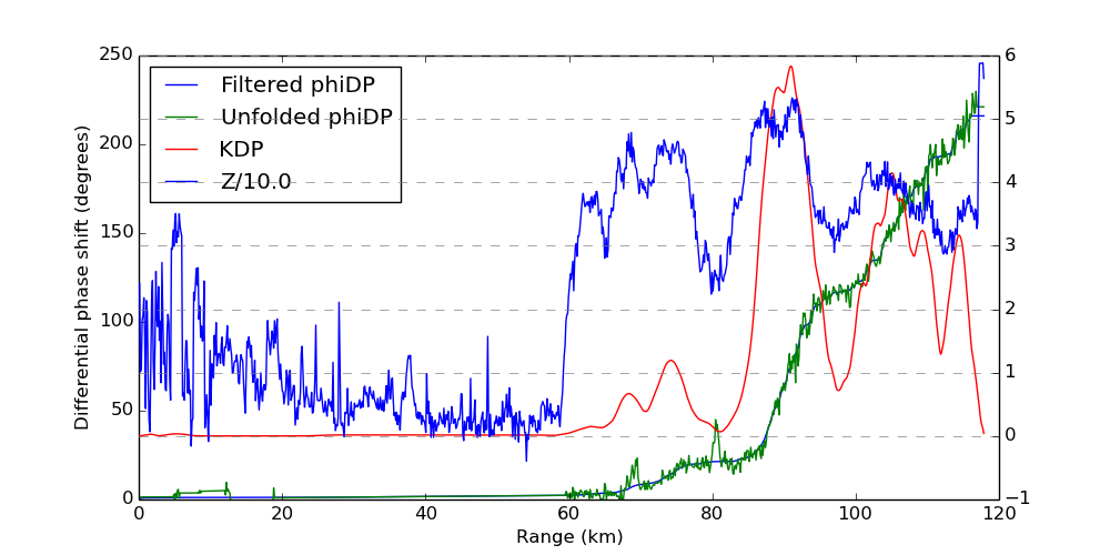
# plot a fields from a single ray
display = pyart.graph.RadarDisplay(radar)
fig = plt.figure(figsize=[10, 5])
ax = fig.add_subplot(111)
ray_num = 191

# filtered phidp and unfolded phidp
display.plot_ray('proc_dp_phase_shift', ray_num, format_str='b-',
                 axislabels_flag=False, title_flag=False, ax=ax)

display.plot_ray('unfolded_differential_phase', ray_num, format_str='g-',
                 axislabels_flag=False, title_flag=False, ax=ax)

# set labels
ax.set_ylim(0, 250)
ax.set_ylabel('Differential phase shift (degrees)')
ax.set_xlabel('Range (km)')

# plot KDP and reflectivity on second axis
ax2 = ax.twinx()
display.plot_ray('recalculated_diff_phase', ray_num, format_str='r-',
                 axislabels_flag=False, title_flag=False, ax=ax2)
radar.add_field_like('reflectivity', 'scaled_reflectivity',
                     radar.fields['reflectivity']['data']/10.)
display.plot_ray('scaled_reflectivity', ray_num, format_str='b-',
                 axislabels_flag=False, title_flag=False, ax=ax2)

# decorate
ax2.yaxis.grid(color='gray', linestyle='dashed')
ax.legend(display.plots,
          ["Filtered phiDP", "Unfolded phiDP", 'KDP', 'Z/10.0'],
          loc='upper left')
plt.show()

Total running time of the example: 177.64 seconds