integration example: integrate_1d

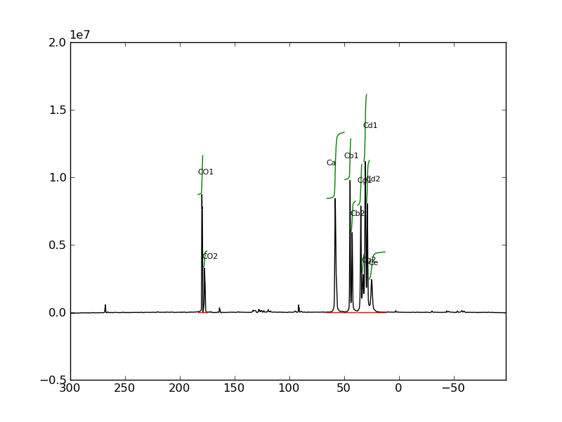
This example shows how to use nmrglue to integrate a 1D NMRPipe spectra. The script reads in ppm peak limits from limits.in and takes a simple summation integral of each peak using the spectra contained in 1d_data.ft. The integration values are writting to area.out and a plot is make showing the integration limits and values overlayed on the spectra to plot.png.

[source code]

#! /usr/bin/env python
# Example scipt to show integration of a 1D spectrum

import nmrglue as ng
import numpy as np
import matplotlib.pyplot as plt

# read in the data from a NMRPipe file
dic,data = ng.pipe.read("1d_data.ft")
length = data.shape[0]

# read in the integration limits
peak_list = np.recfromtxt("limits.in")

# determind the ppm scale
uc = ng.pipe.make_uc(dic,data)
ppm_scale = np.linspace(uc.ppm(0),uc.ppm(data.size-1),data.size)

# plot the spectrum
fig = plt.figure()
ax = fig.add_subplot(111)
ax.plot(ppm_scale,data,'k-')

# prepare the output file
f = open("area.out",'w')
f.write("#Name\tStart\tStop\tArea\n")

# loop over the integration limits
for name,start,end in peak_list:
    min = uc(start,"ppm")
    max = uc(end,"ppm")
    if min>max:
        min,max = max,min

    # extract the peak
    peak = data[min:max+1]
    peak_scale = ppm_scale[min:max+1]

    # plot the integration lines, limits and name of peaks
    ax.plot(peak_scale,peak.cumsum()/100.+peak.max(),'g-')
    ax.plot(peak_scale,[0]*len(peak_scale),'r-')
    ax.text(peak_scale[0],0.5*peak.sum()/100.+peak.max(),name,fontsize=8)

    # write out the integration info
    tup = ( name,peak_scale[0],peak_scale[-1],peak.sum() )
    f.write("%s\t%.3f\t%.3f\t%E\n"%tup)

# close the output file and save the plot
f.close()
ax.set_xlim(ppm_scale[0],ppm_scale[-1])
fig.savefig("plot.png") # change this to plot.pdf, plot.ps, etc

[input file]

#Peak   Start   Stop
CO1     183.40  178.97
CO2     178.97  175.33
# Now some more
Ca      65.77   49.46
Cb1     49.46   43.75     
Cb2     43.75   39.00
Cg1     37.73   33.86
Cg2     33.86   32.00
Cd1     32.00   29.62
Cd2     29.62   26.98
Ce      26.98   12.10

Results:

[output file]

#Name	Start	Stop	Area
CO1	183.395	178.976	2.884854E+08
CO2	178.976	175.333	1.205766E+08
Ca	65.774	49.457	4.906673E+08
Cb1	49.457	43.750	3.062952E+08
Cb2	43.750	38.991	2.336557E+08
Cg1	37.729	33.868	3.073099E+08
Cg2	33.868	31.998	1.470495E+08
Cd1	31.998	29.618	4.963560E+08
Cd2	29.618	26.972	3.168956E+08
Ce	26.972	12.111	2.024605E+08

[figure]